Price formation in agent-based financial markets

In a previous article, I described a very simple agent-based market model. Today, I will revisit the simplistic mechanism for finding the market price by introducing the logic of a price function.

In the original model, the price of an asset is determined by solving all the orders of the orderbook. This means that when the highest bid is higher than the lowest ask—someone offers as much or more than someone else wants for it—a transaction occurs. This process repeats itself until no transaction can occur. The price is then set to the lowest ask: the lowest price for which someone would be willing to sell the asset.

This model simulates a peer-to-peer market. However, most markets (e.g. stock markets) function differently.

Introducing the market maker

The main difference is the introduction of a ‘market maker,’ who buys and sells the assets from investors. This has a number of benefits:

A market maker is always ready to buy or sell an asset. This makes it easier for traders to quickly find someone to trade with. The market moves faster and feels more active.
Without a market maker, the gap between what buyers want to pay (bid price) and what sellers want to sell for (ask price) can be large. Market makers narrow this gap, making it cheaper and easier to trade.
Market makers often help reduce big price jumps or drops by continuously buying and selling, which keeps prices more stable.

So how does it work?

In its most simple form, we can perceive how two types of agents are trading on a market: the investor and the market maker. The investor places an order, which is always filled by the market maker. However, the price at which the orders are filled is determined by the market maker.

The market maker has to balance supply and demand in order to achieve the benefits listed before. So, when there are more bids than asks (more demand than supply), the fill price goes up. Conversely, when the supply is higher, the fill price goes down.

The exact fill price is determined by a so-called market impact function. In this function, the market maker has to balance several things: inventory balance, market volatility, order flow information, competitive pressures, transaction costs and regulatory constraints. So, to manage risk, remain profitable, and stay competitive, he or she may apply a wide range of strategies—a wide variety of (exceedingly complex) market impact functions.

A simple price impact function

Below I show a very basic price impact function as presented in a paper by J. Doyne Farmer¹ over two decades ago.

$P_{t+1} = P_{t} * e^{\frac{\omega}{\lambda}}$

Here, $P_{t+1}$ is the new price and $P_{t}$ the old price. $\omega$ is the net order, so the number of bids minus the number of asks. $\lambda$ Is a scale factor that normalises the order size: the order size that will cause the price to change by a factor of $e$ . In the paper the latter is also called the ‘liquidity.’

Let’s see what that all means using an example.

Let’s say there are 20 agents (investors) in a market, all trying to buy and sell one unit of an asset A, with a starting price of €10.

If, given that price, 10 agents want to buy, and 10 agents want to sell the asset, there is no need to change the price. Indeed, when this is the case, the net order equals 0, and since $e^0$ equals $1$ , the new price is equal to the old price.

Let’s now say there is a mismatch in the market: 11 investors want to buy the asset, and 9 investors want to sell—demand is higher than supply. In this case, we expect the fill price to increase slightly. Let’s calculate this with $\lambda$ equals 5:

$P_{t+1} = 10 * e^{\frac{11-9}{5}}$

$P_{t+1} = 10 * 1.492 = 14.92$

This appears to be a significant price increase (49%) for a relatively small mismatch between supply and demand. In this case, we can say that the market maker is oversensitive to the demand function. Price stability will be hard to maintain.

However, we can change the value of $\lambda$ to reduce this effect. Again, $\lambda$ is the order size that will cause the price to change by a factor of $e$ . Let’s assume that the total number of issued shares is equal to 10,000. We could conceive a rule that a factor $e$ price change is appropriate when the mismatch in supply and demand is equal to 1% of the total shares (i.e. 100).

When we take this as a rule of thumb, the result is different:

$P_{t+1} = 10 * e^{\frac{11-9}{100}}$

$P_{t+1} = 10 * 1.02 = 10.20$

And when supply exceeds the demand:

$P_{t+1} = 10 * e^{\frac{9-11}{100}}$

$P_{t+1} = 10 * 0.98 = 9.80$

Note that the function is exponential, so that the price effect is amplified exponentially for growing imbalances in the market.

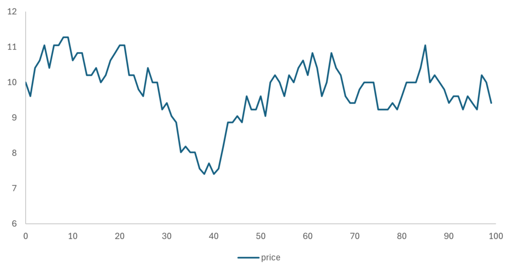
When we put the above example in a model, and we let the 20 agents put randomly a buy (50% chance) or sell (50% change) order over a timespan of 100 cycles. We get the following price movement:

The price appears to move in a random walk, which makes sense since the net order flow (supply and demand) is also based on a random function.

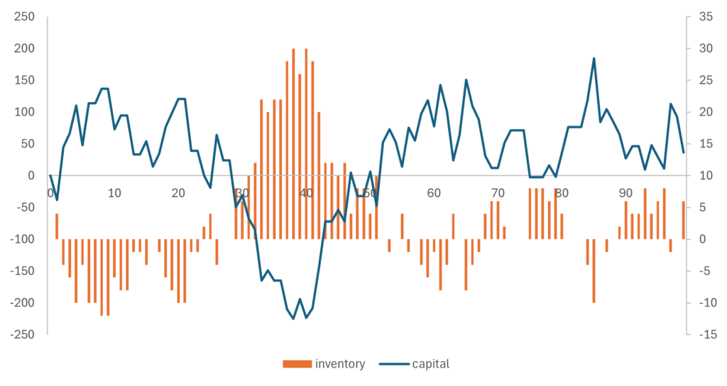
More interesting is the situation for the market maker, because it is important that he or she can maintain a sustainable position:

While it may look a little complicated, the graph makes perfect sense: when inventory (orange bars, right axis) of the market maker goes down, he or she has sold off assets. Hence, its capital (blue line, left axis) should go up. When inventory goes up, the effect is reversed.

It seems that with this very basic price impact function, we can easily simulate a more realistic agent-based market model.

Footnotes

Farmer, J. D. (2000). Market force, ecology, and evolution. 66.

Leave a Reply Cancel reply

PAGE CONTENTS

PAGES
home
about me
contact

BLOGS
a new-age finance
personal growth
bits & pieces
the green zone
summaries